Tutorial II. An Enrichment Exercise

• How many terms of the McLaurin series are required to provide an approximation for the sine function?
  (The McLaurin series for the sine function is x-x³/3!+x⁵/5!-x⁷/7!+x⁹/9!-x¹¹/11!+....)

From the form of the McLaurin series, we can deduce that, ultimately, each successive term of the series brings us closer to the limiting value, on alternate sides. We will take a finite prefix of the McLaurin series as an approximation to the sine function: the more terms we take, the closer the approximation. Our question is: How many terms would be required?

Plot the sine function and the McLaurin polynomial simultaneously
To visualize and better understand the situation, we will plot the sine function and the McLaurin polynomial simultaneously.

1. Launch GrafEq by double clicking its icon.

2. Click on the title splash screen to proceed - the screen will disappear, and the Graph #1 Relation #1 input window will open automatically.

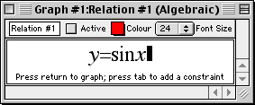
3. Enter the sine function relation in the relation input window, as in figure II.1 following:
   
   Figure II.1: The sine function relation
   

4. Go on to the Create View window by pressing return from within the relation window.

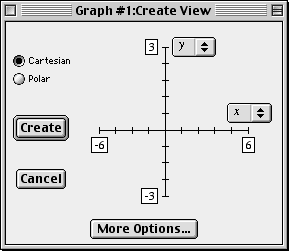
5. The Create View window will appear; the default mode (Cartesian) is fine, but the bounds of the axes can be adjusted to obtain a more relevant and focused view of (-6, 6) by (-3, 3), as seen in figure II.2 following:
   
   Figure II.2: Default view bounds changed
   
   • For the y-axis bounds:
     • click on the upper bound box and change 10 to 3; and
     • click on the lower bound box and change -10 to -3.
   • For the x-axis bounds:
     • click on the upper bound box and change 10 to 6; and
     • click on the lower bound box and change -10 to -6.

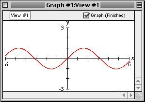
6. Click on the Create button; GrafEq will plot the sine graph as in figure II.3 following:
   
   Figure II.3: The sine graph
   

7. Now open a new relation input window to enter the McLaurin polynomial relation.
   1. Choose Graph from the GrafEq main menu; then
   2. choose New Relation.

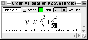
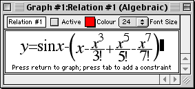
8. In the Relation #2 input window, enter the 3-term McLaurin polynomial relation for the sine function, by typing in “y=x-xup arrow3/3!+xup arrow5/5!”. The entry will be formatted, as seen in figure II.4 following:
   
   Figure II.4: The McLaurin polynomial relation
   

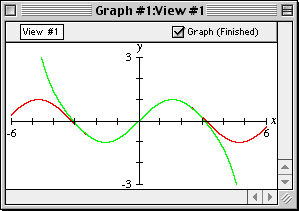
9. Press return, GrafEq will display both relations simultaneously.
   
   Figure II.5: The sine and McLaurin graph
   

Add more terms to the McLaurin series
Next we will look at how adding more terms to the McLaurin series helps the approximation.

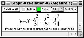
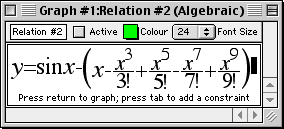
1. Double click on the Relation #2 input window, and add a fourth term to the McLaurin series as in figure II.6 following:
   
   Figure II.6: A 4th-term added to the McLaurin polynomial
   

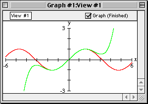
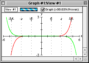
2. Press return and see from the graph, as in figure II.7 following, that the fourth term of the McLaurin series extends the approximation domain from (-2,2) to (-3,3).
   
   Figure II.7: Approximation domain extended from (-2,2) to (-3,3)
   

3. To see the effects of adding more terms to the McLaurin series, repeat the steps as described above.

REVELATIONS:

With each term added, the domain of approximation is further extended. Nevertheless, rather than adding many terms to the McLaurin series, we will take a second look at the sine function and its approximation; note that

• The sine curve is periodic; a single period is sufficient to replicate the entire curve.
• It has odd symmetry about x=0, and even symmetry about x=p/2; its entirety can actually be determined from just one quarter of a period, from 0 to p/2.
• Therefore, we do not need to approximate the sine function over its complete domain; rather, we only need an accurate approximation over the domain of (0,p/2).
• It can be proved that the error of McLaurin approximation for the sine curve increases as the magnitude of x increases. Within the domain of (0,p/2), the maximum error is at p/2.

Find the error of approximation
Although the graphs we have seen of the sine function and McLaurin polynomial seem to coincide at x=p/2, a closer look with GrafEq will help us see that it is actually an approximation.

1. We will first introduce some custom ticks, on the x-axis, in multiples of p/2:
   1. Choose Graph from the GrafEq main menu; then, choose New Custom Ticks.
   2. When the system asks if you want preformated ticks, click the Yes button.
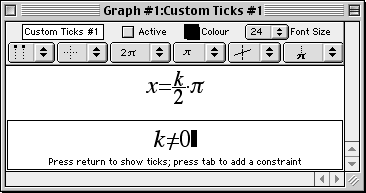
   3. Then, check the option for “multiples of p/2 along x-axis”, and the option for “Excluding x=0”; the custom ticks window will appear as in figure II.8 following:
      
      Figure II.8: Custom ticks in multiples of p/2
      

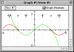
   4. Finally, click the Create button to introduce the ticks to the graph, as seen in figure II.9 following:
      
      Figure II.9: Custom ticks introduced to graph
      

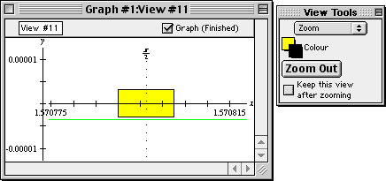
2. Next, we will zoom way in to find the approximation error:
   1. Return to the view buddy, and enter Zoom mode by selecting Zoom from the mode pop-up menu on the top of the floating window.
   2. Since we have to zoom way in to see the error, we will expedite the zooming process - press the left arrow and down arrow keys, to reduce the size of the zoom box, for focused zooming.
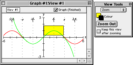
   3. Place the zoom box on the curves, and where x=p/2, as in figure II.10 following:
      
      Figure II.10: Zoom box on the curves, and where x=p/2
      

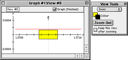
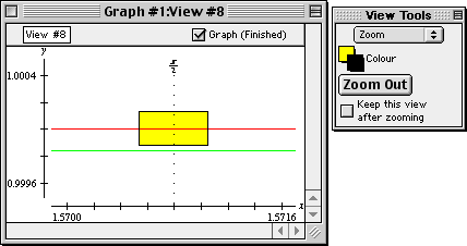
   4. When the zoom box covers the curves where x=p/2, press return to zoom in. Repeat zooming until the two curves are visually separated.

      Hint: The exact picture after zooming depends on where the zoom box is placed at each zoom; therefore, the pictures produced will most probably be a little different every time. Figure II.11 following will serve as an example only.

      
      Figure II.11: Sine and McLaurin curves visually separated
      

3. Now we will read the amplitude of the error; using GrafEq’s One Point view buddy to read the coordinates of the two curves at p/2, then calculate the difference in their y coordinates to get the error.
   1. Return to the view buddy, and enter One Point mode by selecting One Point from the mode pop-up menu on the top of the floating window.
   2. Place the mouse close to the desired point on the graph; pin down the point with the help of the magnified view on the view buddy.
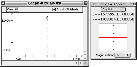
   3. Read the y-coordinate of the sine curve point from the view buddy, which is 1.0000024, as seen in figure II.12 following:
      
      Figure II.12: One-point on sine curve reading 1.0000024
      

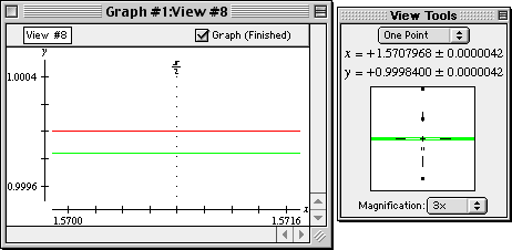
   4. Read the y-coordinate of the McLaurin curve point from the view buddy, which is 0.9998400, as seen in figure II.13 following:
      
      Figure II.13: One-point on McLaurin curve reading 0.9998400
      

   5. The approximation error with a 4-term McLaurin polynomial is therefore: 1.0000024 - 0.9998400, or 0.0001624.

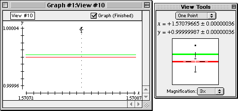
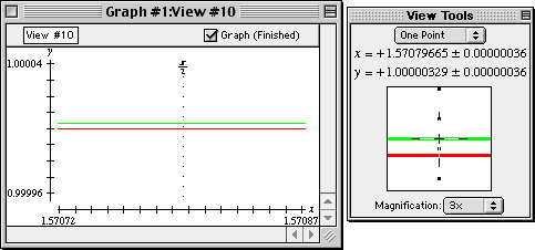
4. Repeat equivalent steps, as described above, for the 5-term McLaurin polynomial, and see that approximation error with a 5-term McLaurin polynomial is: 1.00000329 - 0.99999987, or 0.00000342.
   
   Figure II.14: One-point on sine curve reading 0.99999987
   
   
   Figure II.15: One-point on McLaurin curve reading 1.00000329
   

Now, it has become clear that the question “How many terms would be close enough?” is rather vague. The best answer is perhaps: “How close is desired?”

Hint: Since the terms of the McLaurin series alternate between positive and negative, the approximation using n terms of the series has maximum error of the (n+1)th term, once the terms are decreasing in magnitude. For x in (0,p/2) this occurs immediately. Therefore, an alternative method for determining the number of terms required for some given accuracy, is to find the smallest n such that: (p/2)n/n! < 1/2(desired accuracy)

Congratulations! You have completed this enrichment exercise. But if you like, feel free to try the following suggestions for further exercises:

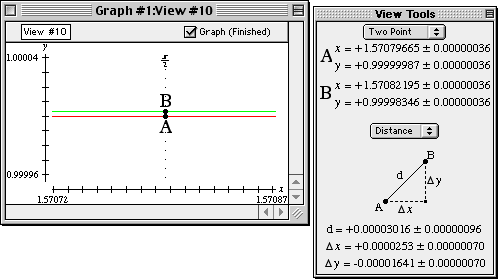
• Discuss the differences among the different methods of reading the error of approximation - besides the one-point method described earlier, other GrafEq features can be used, such as the two-point method.

  From GrafEq’s Two Point view buddy, drag points A and B respectively at the two curves and where x=p/2, as seen in figure II.16 following, then read the distance between the two points from the view buddy.

  
  Figure II.16: Approximation error - two-point method
  

• Graphing the difference of the McLaurin polynomial approximation and the sine function is yet another method for determining the error. We open a new graph to investigate this method.

  Hint: Before opening a new graph, it is good practice to close any current graphs which are not in use to free up the computer’s memory and screen space. Just choose Close Graph from GrafEq’s main File menu.

  • Under the File menu select New Graph.
  • Enter the error for 4-term McLaurin polynomial approximation as Relation #1, and the error for the 5-term McLaurin polynomial approximation as Relation #2, as seen in figure II.17 following:
    
    Figure II.17: Approximation error with 4-term and 5-term McLaurin polynomials
    

  • The error graph should appear as follows:
    
    Figure II.18: Graph of the approximation errors
    

  • And if we zoom in, we can see that the approximation errors are different with the 4-term and 5-term McLaurin polynomials, as seen in figure II.19 following:
    
    Figure II.19: Graph of the approximation errors
    

  • Further, if we zoom in a few more times from figure II.19, we will also see that there is error with the 5-term McLaurin polynomial approximation too, as shown in figure II.20 following:
    
    Figure II.20: Graph of the approximation errors
    

• Express sin10, sin(2p+1), and sin(-p) in terms of values between 0 and p/2.
• Prove that the error of McLaurin approximation for the sine curve increases as the magnitude of x increases.

• For a general description for the GrafEq program, visit the on-line description page at http://www.peda.com/grafeq/.
• For an overview of the program’s functionalities, visit the on-line specifications page at http://www.peda.com/grafeq/.
• For a complete reference, consult the GrafEq manual.
• The appendices provide a useful summary and reference.

• This tutorial is based on GrafEq 2.04; users of other versions of GrafEq might need to adjust some steps for any differences in the user interface.
• While the steps shown in this tutorial are usually the most basic and intuitive ones, GrafEq can be operated with many powerful shortcut keys. Refer to the manual’s appendix of shortcut keys for details.
• Many other features remain to be explored, such as:
  • copying and pasting relations and graphs,
  • making pages for printing,
  • saving graphs to disk,
  • using custom ticks,
  • using one-key short-cuts, and
  • customizing GrafEq for subsequent sessions.

Navigation Options jump up to the Table of Contents go back to A Beginner’s Guided Tour review An Enrichment Exercise continue on to Korte Rondleiding voor beginners (Dutch Tutorial) send us email